Training and Loss

Training a model simply means learning (determining) good values for all the weights and the bias from labeled examples. In supervised learning, a machine learning algorithm builds a model by examining many examples and attempting to find a model that minimizes loss; this process is called empirical risk minimization.

Loss is the penalty for a bad prediction. That is, loss is a number indicating how bad the model’s prediction was on a single example. If the model’s prediction is perfect, the loss is zero; otherwise, the loss is greater. The goal of training a model is to find a set of weights and biases that have low loss, on average, across all examples. For example, Figure 3 shows a high loss model on the left and a low loss model on the right. Note the following about the figure:

• The red arrow represents loss.
• The blue line represents predictions.

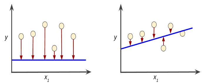Notice that the red arrows in the left plot are much longer than their counterparts in the right plot. Clearly, the blue line in the right plot is a much better predictive model than the blue line in the left plot.

Squared loss: a popular loss function

The linear regression models we’ll examine here use a loss function called squared loss (also known as L2 loss). The squared loss for a single example is as follows: Mean square error (MSE) is the average squared loss per example. To calculate MSE, sum up all the squared losses for individual examples and then divide by the number of examples: 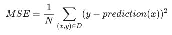where:

• (x,y) is an example in which x is the set of features that the model uses to make predictions and y is the examples label
• prediction (x) is a function of the weights and bias in combination with the set of features x
• D is data set containing many labeled examples, which are (x,y) pairs.
• N is the number of examples in D

Although MSE is commonly-used in machine learning, it is neither the only practical loss function nor the best loss function for all circumstances.